Bayes Report - A Hugo website

Intro Paragraph

“Well hit down the left-field line, and gone!! The winners and still champions, the Toronto Blue Jays.” -Sean McDonough, CBS 1993

This was the call for the 1993 World Series where Joe Carter hit a home run to win the world series. Baseball has been filled for over a century of calls just like this, and has spanned many different periods of baseball. Now-a-days baseball is filled with data and analytics. One of the most interesting things for a lot of people is being able to predict who wins the game. There are many ways to do this. We are looking at predicting the final score based on the inning and the number of runs scored in that inning by both teams.

So, our research question is:

-Can we model the final score of a baseball game by using the number of runs scored in each inning and updating every time an inning is completed?

Literature Review

Given the breadth of data out there for baseball, it is no wonder that there is a lot of literature out there about prediction, and it is also a hot topic for dissertations.

There are a lot of different models out there already, most notably fivethirtyeights elo rating system which is also what they use to predict baseball game outcomes. There model uses data from every year available from retrosheet to create a baseball model that measure how good a baseball team is. Then they added park, travel, rest, and pitcher factors to come up with a prediction for each game. The outcome of the game then influences the rating of each team afterwards (JayBoice 2018). This screams of a Bayesian model, and it is a really good model. However, this uses each game as another data point to determine the posterior distribution.

Aspiring Ph.D’s have used discrete state markov chains to predict win outcomes (Smith Z.J. 2016). Some have used machine learning models to predict future individual player performance (Lyle, A 2007). Which also shows how expansive the mass of data for baseball allows people to be. Smith’s dissertation has every individual plate appearance be a new data point, which would make things really computationally inefficient, and we think fivethirtyeight can be broken down more, so we settled on using each inning as a new point of data to update our hierarchical bayesian model.

Data Description

Our data is game logs for Major League Baseball from the years 2010 - 2018 from retrosheet.org. We searched for the most accurate game logs that contained the number of runs scored in each inning, and retrosheet had both the most, by going all the way back to the 1800’s and the most accurate game logs out there.

The information used here was obtained free of charge from and is copyrighted by Retrosheet. Interested parties may contact Retrosheet at “www.retrosheet.org”.

Current Code Book

Name	Meaning
Date	The date of the game in the form ######## (Day Month Year)
LengthOfGame	The total number of outs made in the game
TimeOfDay	The time of the day the game was played in (Night or Day)
VisitingTeam	The Visiting Team
HomeTeam	The Home Team
VisitingTeamLeague	The Visiting teams league (AL or NL)
HomeTeamLeague	The Home teams league (AL or NL)
VisitingTeamGameNumber	How many games the visiting team has played
HomeTeamGameNumber	How many games the home team has played
VisitingTeamScore	The number of runs scored at the end of the game by the visiting team
HomeTeamScore	The number of runs scored at the end of the game by the home team
VisitingLineScore(2)	The compilation of the number of runs scored in each inning by the visiting team
HomeLineScore(2)	The compilation of the number of runs scored in each inning by the home team
VisitingInningi	The number of runs scored in inning i by the visiting team
HomeInningi	The number of runs scored in inning i by the home team

Data cleaning Code

library(dplyr)
library(ggplot2)
library(rjags)
library(repmis)
library(rsconnect)

gamelogs<-source_data("https://raw.githubusercontent.com/tshogren/Bayesian-Data/master/data_for_dylan.csv")

gamelogs <- gamelogs %>%
  select(-V1)

dataStacked <- data.frame(stack(gamelogs[16:ncol(gamelogs)]))

Data Visualizations

We expect most teams to score 0 or 1 runs per inning, with multiple runs occurring at a lower rate. The first visualization shows the distribution of runs scored by one team in an inning with a poisson distribution overlayed using the average number of runs scored per inning. This depicts how we are looking to determine the number of runs scored per inning, which will then be translated to the team level. We also expect the final score of games to have a similar distribution. This is shown in the next two visualizations. These plots depict the distribution of runs scored in a game for the home team and the visiting team respectively with another poisson model overlayed using the average number of runs scored in the game for the home and the visiting team respectively. Finally, we wanted to look at how these two values interacted with each other. The last visualization depicts how the scores from the home and visiting teams interact. It shows the frequency of final scores between the two teams.

ggplot(dataStacked,aes(x=values))+
  geom_histogram(color = "black", binwidth = 1, aes(y = ..density..))+
  ggtitle("Runs Scored Per Inning")+
  xlab("Runs")+
  stat_density(fun=dpois,args=list(lambda=mean(dataStacked$values)),color="red",geom = "smooth",bw=1)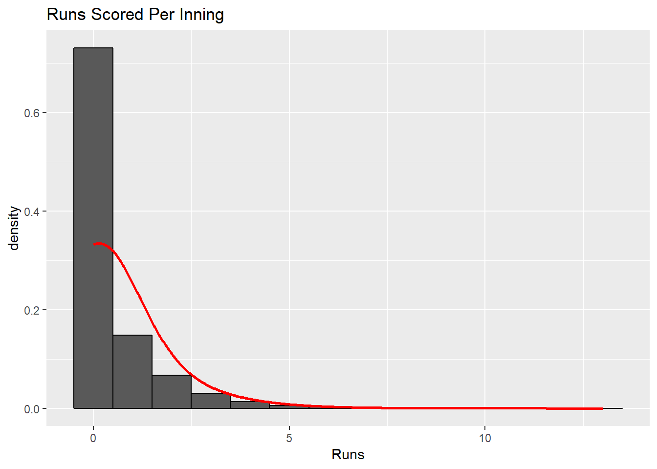

ggplot(gamelogs,aes(x=HomeTeamScore))+
  geom_histogram(color = "black", binwidth = 1, aes(y = ..density..))+
  ggtitle("Runs Scored By Home Team")+
  stat_density(fun=dpois,args=list(lambda=mean(gamelogs$HomeTeamScore)),color="red",geom = "smooth",bw=1)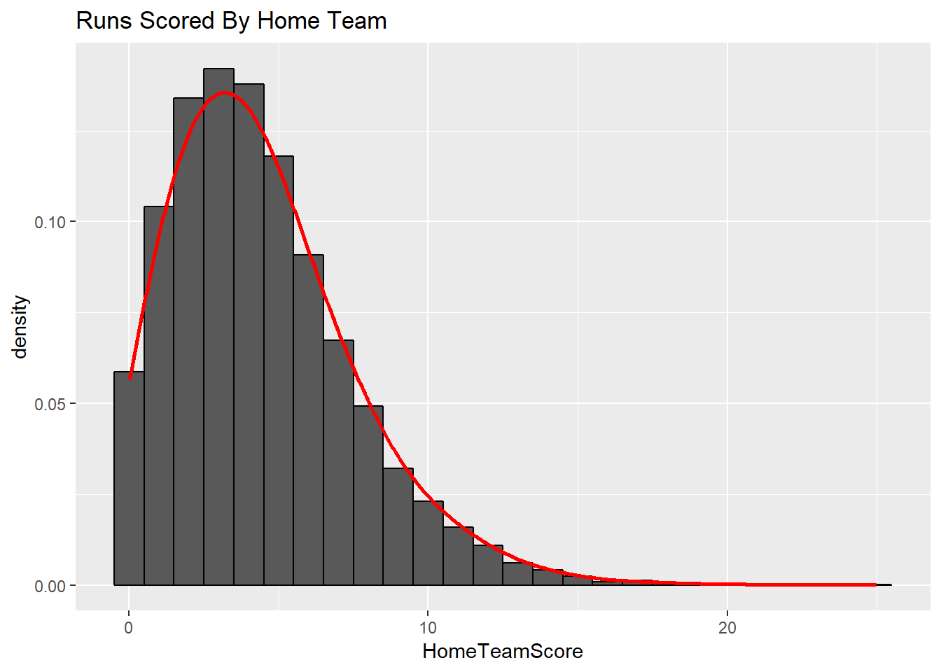

ggplot(gamelogs,aes(VisitingTeamScore))+
  geom_histogram(color = "black", binwidth = 1, aes(y = ..density..))+
  ggtitle("Runs Scored By Visiting Team")+
  stat_density(fun=dpois,args=list(lambda=mean(gamelogs$VisitingTeamScore)),color="red",geom = "smooth",bw=1)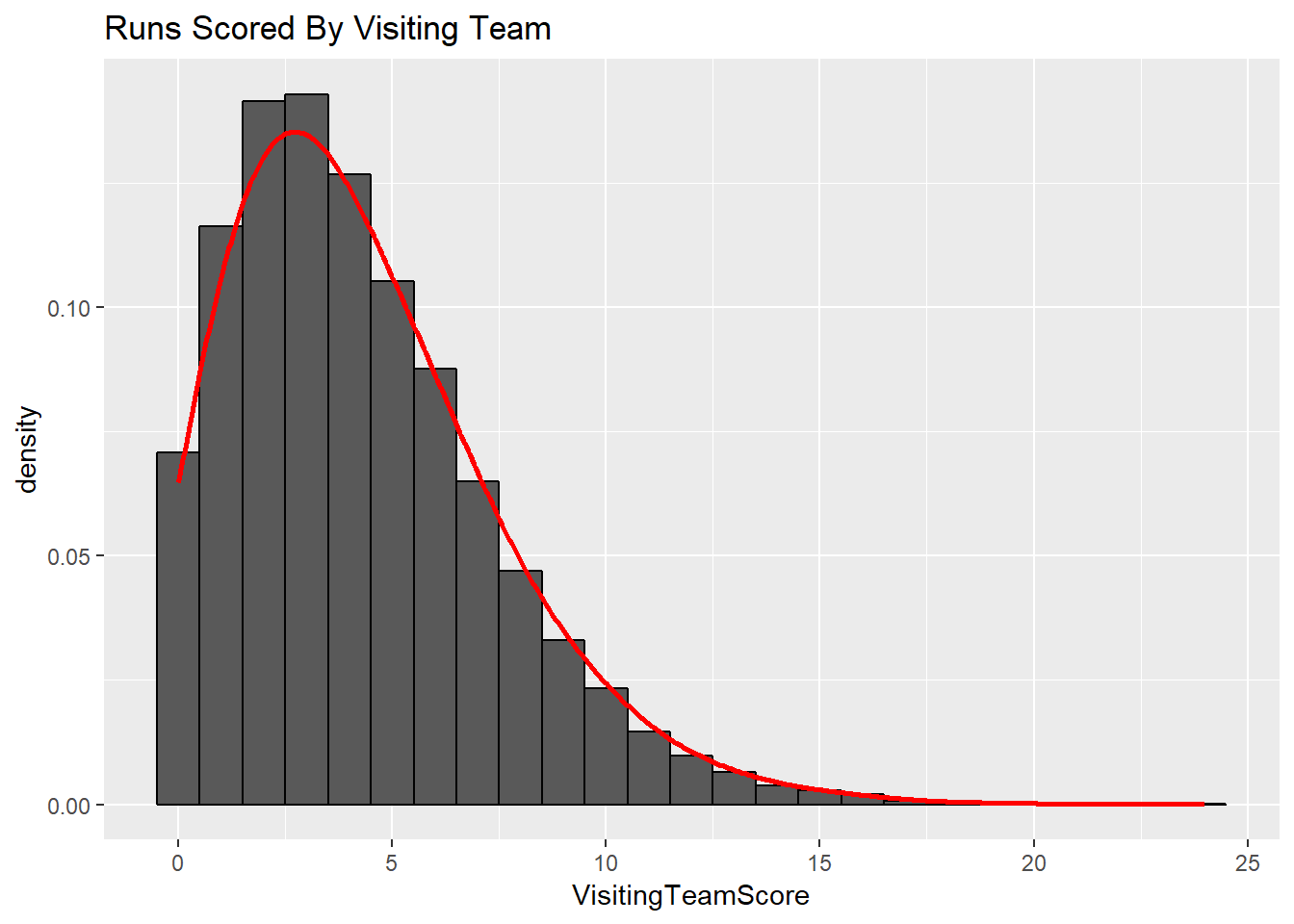

ggplot(gamelogs,aes(HomeTeamScore,VisitingTeamScore))+
  geom_count()+
  ggtitle("Distribution of Game Scores")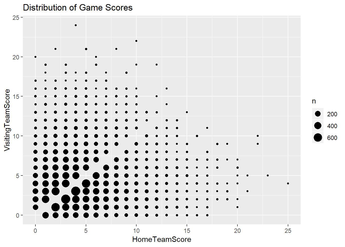

Bayes Models

Bayes Model 1

Our first model is predicting the final score of a game for the visiting team based on the score of the visiting team in the first inning. x is the number of runs scored by the visiting team in the first inning.

$S$ ~ $P o i s (λ)$

$l n (λ) = β_{0} + β_{1} x$

$β_{0}$ ~ N(0,1/100000)

$β_{1}$ ~ N(0,1/100000)

S=Projected number of runs for visiting team at end of game

x= # runs scored in first inning

$β_{0}$ & $β_{1}$ are just vague priors.

This model shows that the amount of runs scored in the first inning by the visiting team has a significant positive effect on the total number of runs scored by the visiting team.

baseballruns_model1.1 <- "model{
    # Data
    for(i in 1:length(y)) {
      y[i] ~ dpois(lambda[i])
      log(lambda[i]) <- beta0+beta1*x[i]

    }

    # Priors
    beta0 ~ dnorm(m0,t0)
    beta1~ dnorm(m1,t1)


}"

baseballruns_jags_1<- jags.model(textConnection(baseballruns_model1.1), 
    data = list(y=gamelogs$VisitingTeamScore,x=gamelogs$VisitingInning1,m0=0,t0=1/100000,m1=0,t1=1/100000),
    inits = list(.RNG.name="base::Wichmann-Hill", .RNG.seed=454))

## Compiling model graph
##    Resolving undeclared variables
##    Allocating nodes
## Graph information:
##    Observed stochastic nodes: 21817
##    Unobserved stochastic nodes: 2
##    Total graph size: 43673
## 
## Initializing model

baseballruns_sim1 <- coda.samples(baseballruns_jags_1,
    variable.names = c("beta0","beta1"),
    n.iter = 10000)

# Store the samples in a data frame:    
baseballruns_chains_1 <- data.frame(iteration = 1:10000, baseballruns_sim1[[1]])

summary(baseballruns_sim1)

## 
## Iterations = 1001:11000
## Thinning interval = 1 
## Number of chains = 1 
## Sample size per chain = 10000 
## 
## 1. Empirical mean and standard deviation for each variable,
##    plus standard error of the mean:
## 
##         Mean       SD  Naive SE Time-series SE
## beta0 1.3341 0.003773 3.773e-05      6.164e-05
## beta1 0.1957 0.002572 2.572e-05      4.169e-05
## 
## 2. Quantiles for each variable:
## 
##         2.5%    25%    50%    75%  97.5%
## beta0 1.3268 1.3315 1.3340 1.3366 1.3416
## beta1 0.1908 0.1939 0.1957 0.1975 0.2007

set.seed(454)
gamelogs2 <- gamelogs %>%
  mutate(VisitorPrediction = rpois(nrow(gamelogs),lambda=exp(1.3341+0.1957*VisitingInning1)))
gamelogs2 %>%
  summarise(mean((VisitorPrediction-VisitingTeamScore)^2),
            mean(VisitorPrediction==VisitingTeamScore))

##   mean((VisitorPrediction - VisitingTeamScore)^2)
## 1                                        12.78636
##   mean(VisitorPrediction == VisitingTeamScore)
## 1                                    0.1180272

ggplot(gamelogs2,aes(x=VisitorPrediction,y=VisitingTeamScore))+geom_point()+geom_abline(intercept = 0,slope=1)+geom_jitter()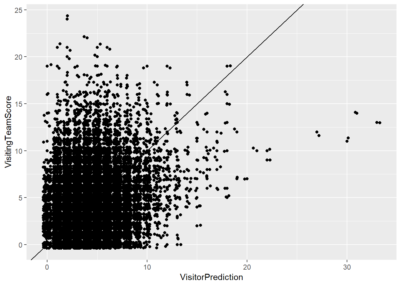

The mean squared error for model 1 is 12.78636 and the prediction is correct 11.80272% of the time. By looking at the plot of the predictions versus the actual scores, we can see that there are some large outliers on both ends of the model. There are a number of games where we predicted the visiting team to score 20 or more runs when they actually scored between 10 and 15 runs. Similarly, there are a large number of games where we project the visiting team to score 5 or less runs, but in reality they scored 10 or more runs.

Bayes Model 2

This model is now taking into account both teams scores through the first four innings. $x + z + q + w$ is the number of runs scored by the visiting team in the first four innings and $(a + b + c + d)$ is the number of runs scored by the home team in the first four innings.

v ~ $P o i s (λ)$

h ~ $P o i s (λ_{2})$

$l n (λ) = β_{0} + β_{1} (x + z + q + w)$

$l n (λ_{2}) = β_{2} + β_{3} (a + b + c + d)$

$β_{0}$ ~ N(0,1/100000)

$β_{1}$ ~ N(0,1/100000)

$β_{2}$ ~ N(0,1/100000)

$β_{3}$ ~ N(0,1/100000)

The number of runs scored by both teams has a positive effect on the total number of runs scored by the team, but the visiting team is expected to score slightly more runs given that both teams have scored and the game is tied or the visiting team is winning. The home team is expected to score more runs if they are leading or the game is tied at zero.

baseballruns_model2.1 <- "model{
    # Data
    for(i in 1:length(v)) {
      v[i] ~ dpois(lambda[i])
      h[i] ~ dpois(lambda2[i])
      log(lambda[i]) <- beta0+beta1*(x[i]+z[i]+q[i]+w[i])
      log(lambda2[i]) <- beta2+beta3*(a[i]+b[i]+c[i]+d[i])
}

    # Priors
    beta0 ~ dnorm(m0,t0)
    beta1~ dnorm(m1,t1)
    beta2 ~dnorm(m2,t2)
    beta3~dnorm(m3,t3)
}"

baseballruns_jags_2<- jags.model(textConnection(baseballruns_model2.1), 
    data = list(v=gamelogs$VisitingTeamScore,x=gamelogs$VisitingInning1,z=gamelogs$VisitingInning2, q=gamelogs$VisitingInning3,w=gamelogs$VisitingInning4,a=gamelogs$HomeInning1,b=gamelogs$HomeInning2,c=gamelogs$HomeInning3,d=gamelogs$HomeInning4, h=gamelogs$HomeTeamScore, m0=0,t0=1/100000,m1=0,t1=1/100000,m2=0,t2=1/100000,m3=0,t3=1/100000),
    inits = list(.RNG.name="base::Wichmann-Hill", .RNG.seed=454))

## Compiling model graph
##    Resolving undeclared variables
##    Allocating nodes
## Graph information:
##    Observed stochastic nodes: 43634
##    Unobserved stochastic nodes: 4
##    Total graph size: 219140
## 
## Initializing model

baseballruns_sim2 <- coda.samples(baseballruns_jags_2,
    variable.names = c("beta0","beta1","beta2","beta3"),
    n.iter = 10000)

# Store the samples in a data frame:    
baseballruns_chains_2 <- data.frame(iteration = 1:10000, baseballruns_sim2[[1]])

summary(baseballruns_sim2)

## 
## Iterations = 1001:11000
## Thinning interval = 1 
## Number of chains = 1 
## Sample size per chain = 10000 
## 
## 1. Empirical mean and standard deviation for each variable,
##    plus standard error of the mean:
## 
##        Mean       SD  Naive SE Time-series SE
## beta0 1.033 0.004708 4.708e-05      1.050e-04
## beta1 0.181 0.001212 1.212e-05      2.690e-05
## beta2 1.053 0.004772 4.772e-05      1.089e-04
## beta3 0.169 0.001120 1.120e-05      2.588e-05
## 
## 2. Quantiles for each variable:
## 
##         2.5%    25%   50%    75%  97.5%
## beta0 1.0235 1.0296 1.033 1.0359 1.0420
## beta1 0.1787 0.1802 0.181 0.1819 0.1834
## beta2 1.0438 1.0499 1.053 1.0564 1.0623
## beta3 0.1668 0.1683 0.169 0.1698 0.1712

set.seed(454)
gamelogs3 <- gamelogs %>%
  mutate(VisitorPrediction = 
           rpois(nrow(gamelogs),lambda=exp(1.033+0.181*(VisitingInning1+VisitingInning2+VisitingInning3+VisitingInning4))),
                 HomePrediction = 
                   rpois(nrow(gamelogs),lambda=exp(1.053+0.169*(HomeInning1+HomeInning2+HomeInning3+HomeInning4))))
gamelogs3 %>%
  summarise(mean((VisitorPrediction-VisitingTeamScore)^2),
            mean((HomePrediction-HomeTeamScore)^2),
            mean(VisitorPrediction==VisitingTeamScore),
            mean(HomePrediction==HomeTeamScore))

##   mean((VisitorPrediction - VisitingTeamScore)^2)
## 1                                        10.19893
##   mean((HomePrediction - HomeTeamScore)^2)
## 1                                 9.639089
##   mean(VisitorPrediction == VisitingTeamScore)
## 1                                    0.1425952
##   mean(HomePrediction == HomeTeamScore)
## 1                             0.1375533

ggplot(gamelogs3,aes(x=VisitorPrediction,y=VisitingTeamScore))+geom_point()+geom_abline(intercept = 0,slope=1)+geom_jitter()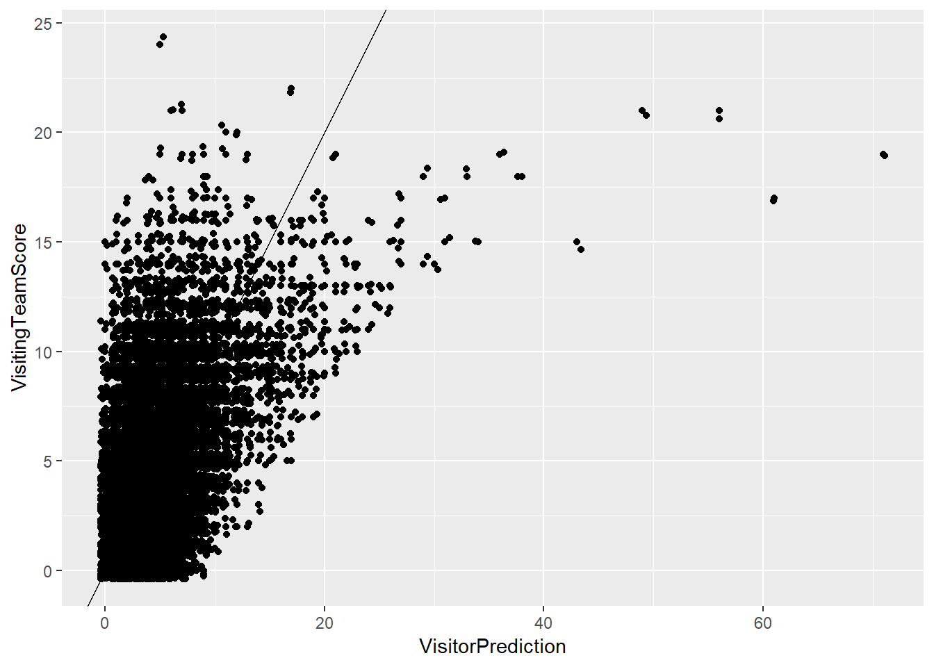

ggplot(gamelogs3,aes(x=HomePrediction,y=HomeTeamScore))+geom_point()+geom_abline(intercept = 0,slope=1)+geom_jitter()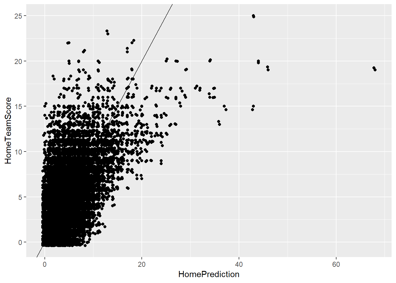

The mean squared error for model 2 is 10.19893 for the visiting team and 9.639089 for the home team. The predictions are correct 14.25952% of the time for the visiting team and 13.75533% of the time for the home team. The mean squared error was lower for the visiting team in this model than it was in the previous model and the model also predicted the score correctly at a higher rate. Although there are fewer large errors in terms of predicted scores versus actual scores, the magnintude of the largest errors increased significantly to almost 50 at the largest.

Bayes Model 3

This model is now taking into account both teams scores through the first four innings and the teams that are playing. $x + z + q + w$ is the number of runs scored by the visiting team in the first four innings and $(a + b + c + d)$ is the number of runs scored by the home team in the first four innings. i is the ith team. Instead of the final score, it is modeling for the amount of runs scored in the remainder of the game.

v ~ $P o i s (λ)$

h ~ $P o i s (λ_{2})$

$l n (λ) = β_{0} + β_{1} (x + z + q + w) + β_{4, i}$

$l n (λ_{2}) = β_{2} + β_{3} (a + b + c + d) + β_{5, i}$

$β_{0}$ ~ N(0,1/100000)

$β_{1}$ ~ N(0,1/100000)

$β_{2}$ ~ N(0,1/100000)

$β_{3}$ ~ N(0,1/100000)

$β_{4, 1}$ = 0

$β_{4, i}$ ~ N(0,1/100000) for i from 2 to 31

$β_{5, 1}$ = 0

$β_{5, i}$ ~ N(0,1/100000) for i from 2 to 31

The number of runs scored by both teams has a positive effect on the total number of runs scored by the team. The Angels are expected to score more runs as the visiting team than other teams holding everything else constant, and the Rockies are expected to score more runs as the home team compared to other teams holding everything else constant.

baseballruns_model4 <- "model{
    # Data
    for(i in 1:length(v)) {
      v[i] ~ dpois(lambda[i])
      h[i] ~ dpois(lambda2[i])
      log(lambda[i]) <- beta0+beta1*(x[i])+beta4[r[i]]
      log(lambda2[i]) <- beta2+beta3*(a[i])+beta5[e[i]]
}

    # Priors
    beta0 ~ dnorm(m0,t0)
    beta1 ~ dnorm(m1,t1)
    beta2 ~ dnorm(m2,t2)
    beta3 ~ dnorm(m3,t3)
    beta4[1] <- 0
    beta4[2] ~ dnorm(m0,t0)
    beta4[3] ~ dnorm(m0,t0)
    beta4[4] ~ dnorm(m0,t0)
    beta4[5] ~ dnorm(m0,t0)
    beta4[6] ~ dnorm(m0,t0)
    beta4[7] ~ dnorm(m0,t0)
    beta4[8] ~ dnorm(m0,t0)
    beta4[9] ~ dnorm(m0,t0)
    beta4[10] ~ dnorm(m0,t0)
    beta4[11] ~ dnorm(m0,t0)
    beta4[12] ~ dnorm(m0,t0)
    beta4[13] ~ dnorm(m0,t0)
    beta4[14] ~ dnorm(m0,t0)
    beta4[15] ~ dnorm(m0,t0)
    beta4[16] ~ dnorm(m0,t0)
    beta4[17] ~ dnorm(m0,t0)
    beta4[18] ~ dnorm(m0,t0)
    beta4[19] ~ dnorm(m0,t0)
    beta4[20] ~ dnorm(m0,t0)
    beta4[21] ~ dnorm(m0,t0)
    beta4[22] ~ dnorm(m0,t0)
    beta4[23] ~ dnorm(m0,t0)
    beta4[24] ~ dnorm(m0,t0)
    beta4[25] ~ dnorm(m0,t0)
    beta4[26] ~ dnorm(m0,t0)
    beta4[27] ~ dnorm(m0,t0)
    beta4[28] ~ dnorm(m0,t0)
    beta4[29] ~ dnorm(m0,t0)
    beta4[30] ~ dnorm(m0,t0)
    beta4[31] ~ dnorm(m0,t0)
    beta5[1] <- 0
    beta5[2] ~ dnorm(m0,t0)
    beta5[3] ~ dnorm(m0,t0)
    beta5[4] ~ dnorm(m0,t0)
    beta5[5] ~ dnorm(m0,t0)
    beta5[6] ~ dnorm(m0,t0)
    beta5[7] ~ dnorm(m0,t0)
    beta5[8] ~ dnorm(m0,t0)
    beta5[9] ~ dnorm(m0,t0)
    beta5[10] ~ dnorm(m0,t0)
    beta5[11] ~ dnorm(m0,t0)
    beta5[12] ~ dnorm(m0,t0)
    beta5[13] ~ dnorm(m0,t0)
    beta5[14] ~ dnorm(m0,t0)
    beta5[15] ~ dnorm(m0,t0)
    beta5[16] ~ dnorm(m0,t0)
    beta5[17] ~ dnorm(m0,t0)
    beta5[18] ~ dnorm(m0,t0)
    beta5[19] ~ dnorm(m0,t0)
    beta5[20] ~ dnorm(m0,t0)
    beta5[21] ~ dnorm(m0,t0)
    beta5[22] ~ dnorm(m0,t0)
    beta5[23] ~ dnorm(m0,t0)
    beta5[24] ~ dnorm(m0,t0)
    beta5[25] ~ dnorm(m0,t0)
    beta5[26] ~ dnorm(m0,t0)
    beta5[27] ~ dnorm(m0,t0)
    beta5[28] ~ dnorm(m0,t0)
    beta5[29] ~ dnorm(m0,t0)
    beta5[30] ~ dnorm(m0,t0)
    beta5[31] ~ dnorm(m0,t0)
}"

baseballruns_jags_4<- jags.model(textConnection(baseballruns_model4), 
    data = list(v=gamelogs$VisitingTeamScore-gamelogs$VisitingInning1-gamelogs$VisitingInning2-gamelogs$VisitingInning3-gamelogs$VisitingInning4,x=gamelogs$VisitingInning1+gamelogs$VisitingInning2+gamelogs$VisitingInning3+gamelogs$VisitingInning4,a=gamelogs$HomeInning1+gamelogs$HomeInning2+gamelogs$HomeInning3+gamelogs$HomeInning4,h=gamelogs$HomeTeamScore-gamelogs$HomeInning1-gamelogs$HomeInning2-gamelogs$HomeInning3-gamelogs$HomeInning4, m0=0,t0=1/100000,m1=0,t1=1/100000,m2=0,t2=1/100000,m3=0,t3=1/100000,r=as.factor(gamelogs$VisitingTeam),e=as.factor(gamelogs$HomeTeam)),
    inits = list(.RNG.name="base::Wichmann-Hill", .RNG.seed=454))

## Compiling model graph
##    Resolving undeclared variables
##    Allocating nodes
## Graph information:
##    Observed stochastic nodes: 43634
##    Unobserved stochastic nodes: 64
##    Total graph size: 132546
## 
## Initializing model

baseballruns_sim4 <- coda.samples(baseballruns_jags_4,
    variable.names = c("beta0","beta1","beta2","beta3","beta4","beta5"),
    n.iter = 10000)

# Store the samples in a data frame:    
baseballruns_chains_4 <- data.frame(iteration = 1:10000, baseballruns_sim4[[1]])

summary(baseballruns_sim4)

## 
## Iterations = 1001:11000
## Thinning interval = 1 
## Number of chains = 1 
## Sample size per chain = 10000 
## 
## 1. Empirical mean and standard deviation for each variable,
##    plus standard error of the mean:
## 
##                Mean       SD  Naive SE Time-series SE
## beta0      0.960415 0.024112 2.411e-04      2.242e-03
## beta1      0.017468 0.002157 2.157e-05      4.328e-05
## beta2      0.761387 0.025383 2.538e-04      2.366e-03
## beta3     -0.003408 0.002072 2.072e-05      4.174e-05
## beta4[1]   0.000000 0.000000 0.000e+00      0.000e+00
## beta4[2]  -0.147895 0.033349 3.335e-04      2.003e-03
## beta4[3]  -0.091924 0.033675 3.368e-04      2.130e-03
## beta4[4]  -0.143701 0.033965 3.397e-04      2.159e-03
## beta4[5]  -0.026175 0.032464 3.246e-04      2.138e-03
## beta4[6]  -0.123760 0.034367 3.437e-04      2.114e-03
## beta4[7]  -0.126596 0.033975 3.398e-04      1.964e-03
## beta4[8]  -0.151881 0.033698 3.370e-04      2.004e-03
## beta4[9]  -0.086370 0.033555 3.356e-04      2.146e-03
## beta4[10] -0.325972 0.035655 3.566e-04      1.967e-03
## beta4[11] -0.123163 0.033522 3.352e-04      2.153e-03
## beta4[12] -0.177787 0.055298 5.530e-04      1.826e-03
## beta4[13] -0.105537 0.033122 3.312e-04      2.045e-03
## beta4[14] -0.164001 0.034151 3.415e-04      2.022e-03
## beta4[15] -0.040364 0.033098 3.310e-04      2.017e-03
## beta4[16] -0.216354 0.036999 3.700e-04      2.080e-03
## beta4[17] -0.146764 0.033744 3.374e-04      2.126e-03
## beta4[18] -0.119476 0.033543 3.354e-04      2.043e-03
## beta4[19] -0.075759 0.033425 3.342e-04      2.122e-03
## beta4[20] -0.077141 0.033222 3.322e-04      2.147e-03
## beta4[21] -0.101590 0.033733 3.373e-04      2.136e-03
## beta4[22] -0.144865 0.033774 3.377e-04      2.087e-03
## beta4[23] -0.151013 0.033724 3.372e-04      2.047e-03
## beta4[24] -0.151600 0.034577 3.458e-04      2.242e-03
## beta4[25] -0.170484 0.033644 3.364e-04      1.972e-03
## beta4[26] -0.135969 0.034455 3.446e-04      2.196e-03
## beta4[27] -0.058339 0.032729 3.273e-04      2.122e-03
## beta4[28] -0.121218 0.033474 3.347e-04      2.176e-03
## beta4[29] -0.159551 0.034554 3.455e-04      2.109e-03
## beta4[30] -0.071936 0.033629 3.363e-04      2.084e-03
## beta4[31] -0.139272 0.033874 3.387e-04      2.074e-03
## beta5[1]   0.000000 0.000000 0.000e+00      0.000e+00
## beta5[2]   0.180789 0.034419 3.442e-04      2.505e-03
## beta5[3]   0.065096 0.035234 3.523e-04      2.261e-03
## beta5[4]   0.150454 0.034303 3.430e-04      2.125e-03
## beta5[5]   0.234412 0.034237 3.424e-04      2.294e-03
## beta5[6]   0.067919 0.035009 3.501e-04      2.222e-03
## beta5[7]   0.116033 0.034608 3.461e-04      2.243e-03
## beta5[8]   0.116985 0.034546 3.455e-04      2.376e-03
## beta5[9]   0.124896 0.034578 3.458e-04      2.327e-03
## beta5[10]  0.358271 0.033190 3.319e-04      2.084e-03
## beta5[11]  0.184371 0.033988 3.399e-04      2.442e-03
## beta5[12]  0.003465 0.059794 5.979e-04      2.331e-03
## beta5[13]  0.002104 0.034916 3.492e-04      2.369e-03
## beta5[14]  0.102180 0.034550 3.455e-04      2.202e-03
## beta5[15]  0.010912 0.035381 3.538e-04      2.335e-03
## beta5[16]  0.010754 0.038202 3.820e-04      2.232e-03
## beta5[17]  0.076230 0.034904 3.490e-04      2.376e-03
## beta5[18]  0.082219 0.035357 3.536e-04      2.495e-03
## beta5[19]  0.192421 0.033798 3.380e-04      2.228e-03
## beta5[20]  0.006187 0.035482 3.548e-04      2.326e-03
## beta5[21]  0.097612 0.034330 3.433e-04      2.241e-03
## beta5[22]  0.041899 0.035546 3.555e-04      2.340e-03
## beta5[23] -0.013310 0.035828 3.583e-04      2.375e-03
## beta5[24] -0.057681 0.035940 3.594e-04      2.401e-03
## beta5[25] -0.107798 0.036658 3.666e-04      2.253e-03
## beta5[26] -0.006729 0.035732 3.573e-04      2.395e-03
## beta5[27]  0.098767 0.035018 3.502e-04      2.266e-03
## beta5[28]  0.023508 0.035307 3.531e-04      2.309e-03
## beta5[29]  0.212612 0.033870 3.387e-04      2.420e-03
## beta5[30]  0.152250 0.034009 3.401e-04      2.275e-03
## beta5[31]  0.116831 0.034861 3.486e-04      2.311e-03
## 
## 2. Quantiles for each variable:
## 
##                 2.5%        25%       50%       75%      97.5%
## beta0      0.9146598  0.9437433  0.960170  0.977508  1.0055418
## beta1      0.0132930  0.0160114  0.017446  0.018935  0.0216703
## beta2      0.7115821  0.7439533  0.761830  0.778221  0.8126252
## beta3     -0.0074125 -0.0048337 -0.003411 -0.002021  0.0007012
## beta4[1]   0.0000000  0.0000000  0.000000  0.000000  0.0000000
## beta4[2]  -0.2141510 -0.1704019 -0.147633 -0.125494 -0.0834582
## beta4[3]  -0.1570972 -0.1143743 -0.091795 -0.069157 -0.0251389
## beta4[4]  -0.2090960 -0.1672101 -0.143968 -0.120952 -0.0759869
## beta4[5]  -0.0888184 -0.0483078 -0.026260 -0.004058  0.0366793
## beta4[6]  -0.1899163 -0.1471731 -0.124167 -0.100432 -0.0562610
## beta4[7]  -0.1920219 -0.1501532 -0.126974 -0.103590 -0.0584057
## beta4[8]  -0.2172106 -0.1747588 -0.151941 -0.129297 -0.0858944
## beta4[9]  -0.1504205 -0.1089345 -0.086499 -0.063501 -0.0192616
## beta4[10] -0.3942989 -0.3499877 -0.326281 -0.301821 -0.2560408
## beta4[11] -0.1890319 -0.1461678 -0.122718 -0.100180 -0.0585745
## beta4[12] -0.2858217 -0.2149578 -0.177882 -0.139631 -0.0712747
## beta4[13] -0.1690583 -0.1285062 -0.105393 -0.083048 -0.0410465
## beta4[14] -0.2298328 -0.1871891 -0.164080 -0.140464 -0.0966135
## beta4[15] -0.1053584 -0.0633474 -0.040550 -0.018049  0.0253920
## beta4[16] -0.2883781 -0.2411479 -0.216267 -0.191721 -0.1438058
## beta4[17] -0.2118687 -0.1699185 -0.146620 -0.124027 -0.0807846
## beta4[18] -0.1856675 -0.1420458 -0.119452 -0.096773 -0.0541902
## beta4[19] -0.1409864 -0.0985176 -0.075761 -0.053634 -0.0094469
## beta4[20] -0.1429828 -0.0992136 -0.077228 -0.054717 -0.0111828
## beta4[21] -0.1670383 -0.1243038 -0.101453 -0.078317 -0.0348634
## beta4[22] -0.2109210 -0.1677935 -0.145266 -0.122066 -0.0792368
## beta4[23] -0.2169549 -0.1739477 -0.150893 -0.128199 -0.0853158
## beta4[24] -0.2185927 -0.1750904 -0.151558 -0.128035 -0.0827852
## beta4[25] -0.2355869 -0.1933400 -0.170678 -0.148106 -0.1041692
## beta4[26] -0.2030574 -0.1593985 -0.135697 -0.113011 -0.0682102
## beta4[27] -0.1217954 -0.0803057 -0.058248 -0.036845  0.0057855
## beta4[28] -0.1867013 -0.1443647 -0.120946 -0.098912 -0.0551618
## beta4[29] -0.2269698 -0.1832997 -0.159744 -0.136224 -0.0910731
## beta4[30] -0.1369319 -0.0944202 -0.072713 -0.049800 -0.0040581
## beta4[31] -0.2044084 -0.1626181 -0.139112 -0.116423 -0.0736139
## beta5[1]   0.0000000  0.0000000  0.000000  0.000000  0.0000000
## beta5[2]   0.1134904  0.1573746  0.180309  0.204119  0.2491679
## beta5[3]  -0.0040428  0.0415885  0.064973  0.088938  0.1340454
## beta5[4]   0.0836896  0.1273845  0.150061  0.173276  0.2187228
## beta5[5]   0.1658727  0.2115444  0.234410  0.257300  0.3006721
## beta5[6]  -0.0002429  0.0446963  0.067424  0.091295  0.1374283
## beta5[7]   0.0465386  0.0929995  0.116206  0.139432  0.1832024
## beta5[8]   0.0489158  0.0938980  0.116688  0.139864  0.1847218
## beta5[9]   0.0563969  0.1015514  0.124899  0.148184  0.1927578
## beta5[10]  0.2928414  0.3358407  0.358541  0.380605  0.4239125
## beta5[11]  0.1179624  0.1610765  0.184291  0.207907  0.2501303
## beta5[12] -0.1161662 -0.0367897  0.003993  0.044746  0.1178522
## beta5[13] -0.0662925 -0.0216795  0.002289  0.025637  0.0707086
## beta5[14]  0.0337982  0.0795553  0.102213  0.125268  0.1698363
## beta5[15] -0.0592701 -0.0128034  0.011212  0.034269  0.0815804
## beta5[16] -0.0642671 -0.0150740  0.010601  0.035954  0.0863564
## beta5[17]  0.0077914  0.0531603  0.076328  0.100340  0.1436914
## beta5[18]  0.0119001  0.0588633  0.082439  0.106598  0.1506851
## beta5[19]  0.1263497  0.1695125  0.192620  0.215063  0.2590243
## beta5[20] -0.0625583 -0.0174776  0.006161  0.029680  0.0769334
## beta5[21]  0.0315730  0.0739372  0.097543  0.120895  0.1663620
## beta5[22] -0.0283319  0.0176779  0.041365  0.066217  0.1105206
## beta5[23] -0.0847287 -0.0373054 -0.013054  0.010812  0.0567844
## beta5[24] -0.1279735 -0.0819840 -0.058143 -0.033315  0.0124048
## beta5[25] -0.1804151 -0.1329984 -0.107102 -0.082901 -0.0361805
## beta5[26] -0.0777727 -0.0310128 -0.006620  0.017348  0.0629078
## beta5[27]  0.0294959  0.0750954  0.098889  0.122838  0.1665880
## beta5[28] -0.0461385 -0.0002268  0.023541  0.047568  0.0929226
## beta5[29]  0.1467396  0.1900904  0.211809  0.235854  0.2777242
## beta5[30]  0.0847859  0.1293545  0.152252  0.175327  0.2193008
## beta5[31]  0.0496666  0.0929990  0.116624  0.140264  0.1863152

gamelogs4 %>%
  summarise(mean((VisitorPrediction-VisitingTeamScore)^2),
            mean((HomePrediction-HomeTeamScore)^2),
            mean(VisitorPrediction==VisitingTeamScore),
            mean(HomePrediction==HomeTeamScore))

##   mean((VisitorPrediction - VisitingTeamScore)^2)
## 1                                        7.456616
##   mean((HomePrediction - HomeTeamScore)^2)
## 1                                 6.942522
##   mean(VisitorPrediction == VisitingTeamScore)
## 1                                    0.1616629
##   mean(HomePrediction == HomeTeamScore)
## 1                             0.1671174

ggplot(gamelogs4,aes(x=VisitorPrediction,y=VisitingTeamScore))+geom_point()+geom_abline(intercept = 0,slope=1,color="red")+geom_jitter()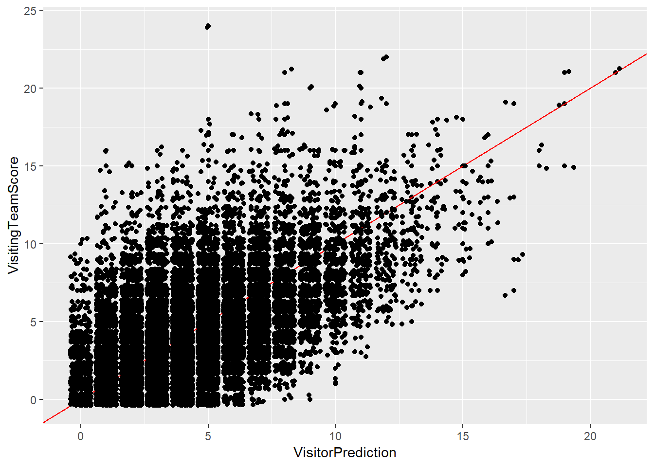

ggplot(gamelogs4,aes(x=HomePrediction,y=HomeTeamScore))+geom_point()+geom_abline(intercept = 0,slope=1,color="red")+geom_jitter()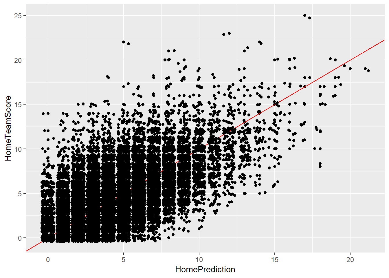

In model 3, we see a large improvement in both mean squared error and correct prediction percentage. For the visiting team, these values were 7.456616 and 16.16629% respectively. For the home team, these values were 6.942522 and 16.71174% respectively. By looking at the graphs, we can see that most of the large outliers were removed and the predictions for the games appear to be reasonable for common scores and most of the higher scores that occur as well.

References

Jayboice. (2018, March 28). How Our MLB Predictions Work. Retrieved May 7, 2019, from https://fivethirtyeight.com/methodology/how-our-mlb-predictions-work/

Lyle, A. (2007). Baseball prediction using ensemble learning (Unpublished doctoral dissertation). University of Georgia.

Smith, Z. J. (2016). A Markov chain model for predicting Major League Baseball (Unpublished doctoral dissertation). University of Texas at Austin. doi:10.15781/T22N4ZP85